Conservation Planning for the Marine Environment

An introduction to tools and techniques

Workshop Data

The data and code for the workshop are available here.

Theory of conservation planning and spatial prioritization

Growing demands for food, energy, and infrastructure put marine ecosystems and their services at risk. To protect marine biodiversity against threats from the accelerating use of the marine environment, international targets aim to expand the global protected area network to 30% of the oceans by 2030. The Kunming-Montreal Global Biodiversity Framework of the Convention on Biological Diversity sets out the 2030 global agenda for nature conservation. Under this framework, 196 countries have committed to protect 30% of the planet through an ecologically-representative, well-connected, and equitably governed system of area-based conservation measures, as well as to restore 30% of degraded ecosystems (Targets 2 & 3) while adapting to climate change. Note that “biodiversity inclusive spatial planning” features prominently in the framework’s Target 1 “Ensure that all areas are under participatory, integrated, and biodiversity inclusive spatial planning and/or effective management processes…”.

In addition, United Nations member states recently adopted a treaty for the conservation and sustainable use of biodiversity in the High Seas, an ambitious goal considering <1% of the High Seas is currently highly protected. Meeting these international targets requires tools and methods that facilitate informed decision-making to balance biodiversity conservation with demands of industries using the environment.

Conservation planning helps stakeholders, the community and planners to work together to identify their resources and accomplish multiple objectives that are best for the land, water, and people (https://marxansolutions.org/whatisconservationplanning/). Conservation planning allows the prioritization of areas important for biodiversity conservation whilst minimizing economic costs, and to quantify ecological and economic impacts of decisions. Conservation planning tools are applicable to a wide range of conservation problems across marine, freshwater and terrestrial ecosystems. These problem can vary in spatial scale, type of biodiversity, managed uses, management actions, and budget. This workshop will teach you the core principles of conservation planning, thus providing the basic hands-on skills to formulate, solve, and interpret conservation problems and their solutions so you can apply conservation planning in your work.

Spatial prioritization refers to quantitative methods that aid in identifying priority areas for a particular action (e.g., conservation) while meeting certain criteria (e.g., meeting area-based targets). In a conservation context, spatial prioritization is used to identify areas for conservation. It is a step in a bigger, more elaborate process called systematic conservation planning that refers to the structured process of identifying, assigning, and monitoring areas for protection, conservation, or restoration. Read more about systematic conservation planning and spatial prioritization in Margules and Pressey (2000) and Tallis et al. (2021).

Important terminology

Here are some key terms that you will need to know to run a prioritization.

Planning region: This is the spatial domain. It is subdivided into planning units.

Planning units: Spatial cells within the planning region, which are usually regular (grids or hexagons) or irregular shapes (e.g., bioregions).

Planning problem: This specifies all the information needed to define a spatial prioritization. This includes the planning region, the planning units, the features, costs, targets, and the objective function.

Solution: The output of the planning problem. Solutions are the protected areas selected. This is either binary (each planning unit is selected (1) or not selected (0) in the reserve system) or can be a proportion of each planning unit

Feature: The elements of interest (e.g., species, habitat, process, cultural site) that you want to protect in the reserve system by setting a target for each.

Target: The minimum quantity or proportion of each conservation feature in the planning region to be included in the solution (e.g., protect 30% of each habitat type in the reserve system).

Cost: Reflects the economic implications of including a planning unit in the reserve (along the coast it could be cost of land acquisition; in the ocean it could be the opportunity cost of lost fisheries revenue). Opportunity costs other than fishing can be included, such as for mining, oil/gas, aggregate extraction and shipping.

Objective function: Specifies the overall goal of a conservation planning problem. All conservation planning problems involve minimizing or maximizing an objective function. The standard objective function in Marxan (and one of the eight objectives in prioritizr) is the minimum set objective, which conserves enough of each feature to meet its target, while minimizing the overall cost of the reserve network.

Common spatial prioritization tools

The most common tools for prioritization are Marxan, Zonation and prioritizr. At their core, these optimization tools all aim to address the conservation planning principles of CARE (Connectivity, Adequacy, Representativeness, Efficiency). Marxan and prioritizr are similar in what they do but differ in how they do it. Zonation is quite different in what it does. Each tool uses different algorithms to solve the conservation planning problem. The Table below is an opinionated summary of the different tools.

Software	Algorithm	Approach	Strengths	Weaknesses
Marxan	Simulated annealing	Uses target-based planning	Free; Easy to use (does not require programming); Widely used; Has spawned more complex relatives that deals with connectivity (MarxanConnect), probability (MarProb), zones (Marxan with Zones)	Approximate solutions; Slow for large problems; Limited ability for customization; Does not allow a workflow from data wrangling to visualization
prioritizr	Integer linear programming	Uses target-based planning	Free; Fast; Solves the exact planning problem; Flexible problem definition; Allows a workflow from data wrangling to visualization; Can handle more complex planning problems than Marxan	Requires knowledge of coding; Fastest solvers are expensive
Zonation	Optimization algorithms	Usually uses non target-based planning	Free; Easy to use (does not require programming); Ranks planning units in terms of their conservation priority	Limited ability for customization; Generally does not satisfy targets at minimum cost; Bespoke graphics but does not allow a workflow from data wrangling to visualization

Introduction to spatial planning with prioritizr

We are going to demonstrate some of the fundamental skills needed in dealing with spatial data based on an example from the Galapagos Exclusive Economic Zone (EEZ). The data used in this workshop are not ours and we attribute the source of the data when we use them. Please also see the Reference section at the end of the notes. This data comes pre-prepared in the correct format. If you would like to see an example of how to create some “fake” data to ensure you can work with your own data when you get home, see Appendix 2.

Study Site - The Galapagos

Today you are a conservation officer helping plan the Galapagos Marine Reserve. The Galapagos Islands and surrounding waters are recognized globally for their unique species and biodiversity, such as the endemic giant tortoises, Galapagos penguins and marine iguanas. In 1998, the Ecuadorian Government created a marine reserve, covering 138,000 km² around the islands, which at the time, made it the second largest marine reserve in the world. However, many of the species inhabiting Galapagos, such as the blue footed booby (Sula nebouxii) and silky shark (Carcharhinus falciformis), utilise the open ocean, and range outside the borders of the reserve. Thanks to tracking studies carried out over the quarter century since the creation of the reserve, we know much more about the movements of many of the species in and around the reserve, and can begin to address the question of whether the current reserve design provides adequate protection for them. We also know much more about the distribution of key ocean habitats in our region. Given that industrial and semi-industrial fishing pressure in Ecuador’s waters outside the reserve increased dramatically at the turn of the century, and that in recent years, large distant water fishing fleets have been reported in the high seas surrounding Ecuador’s Exclusive Economic Zone, the residents of Galapagos are concerned that the existing reserve may not provide sufficient protection to the ocean and wildlife that their livelihoods depend on. They are campaigning for an expansion of the reserve, and have asked us to identify key areas that should be included in their proposed new design. However, the fleets operating around the reserve are concerned that increasing the size of the reserve may affect their livelihoods. In addition to information on key habitats and species movements, we have obtained spatially explicit catch data from the two main fleets - the industrial tuna purse seine fleet and the national longline fleet for large pelagic species.

Loading preliminaries

It is best practice to load and define all “preliminaries” at the start of your R script. These preliminaries range from R packages to variables used across the R script, but typically it encompasses anything and everything that is used and reused throughout the R script.

First, we load the necessary R packages. A really good R package to install the versions of the R packages that are in CRAN is pacman. We are going to install and load packages throughout the course of this workshop, but a common best practice is to install and load all necessary packages to run each script at the top of the R script.

install.packages("pacman")

Load the required packages and code. The code are custom utility functions that we have written to help automate certain tasks.

pacman::p_load(tidyverse, sf, rnaturalearth, patchwork, prioritizr, viridis)
source("utils-functions.R")

Another best practice is to define the input paths as a variable to enhance the reproducibility of your R script. A good R package that breaches the difficulty of setting file paths in different Operating Systems (e.g., Windows syntax vs Mac), among other cool things, is the here R package. If you want to read more about the functionality of this package, take a look at their website.

inputDat <- file.path("Input") # Define file paths

Next, we define the Coordinated Reference System (CRS) that will be used throughout this R script. There are different ways to do this, but the two most common ones are using the EPSG code and the PROJ4 strings. Here’s a pdf that was prepared by M. Frazier and is freely available online that clearly explains the CRS syntax well. It is recommended to use the EPSG code or WKT (Well Known Text), but we find that using the PROJ4 string version of the CRS is useful for plotting maps that are not necessarily centered in the Meridian. But note PROJ4 is technically deprecated now so use with care.

Define CRS as the Mollweide Projection

cCRS <- "ESRI:54009" 

Types of Spatial Data

To save time, we have pre-prepared the data for this workshop, but here we provide a brief overview of the types of data you will see, and the packages you can use to process them. Spatial data usually takes one of two forms — vector or raster.

Vector data is represented as points, lines, or polygons. Raster data is represented in grids of cells (i.e., pixels). There are pros and cons to each of the data formats, but the beauty of dealing with spatial data in R is that you can easily convert between the two forms of spatial data. Here, we show how you can load vector and raster data saved in different file formats. Vector data is usually saved as a shapefile (.shp) and attached to this are other files that contain the metadata (e.g., .shx, .dbf). All of these are usually in one folder. A useful R package to wrangle vector files is the sf R package. It is worth familiarizing yourself with this package.

Raster data is usually saved as a GeoTIFF (Geo Tagged Image File Formats; .tiff). Another file format that is really good at compressing/storing large amounts of data is the netCDF (Network Common Data Form; .nc).
A useful R package for wrangling raster files (and also vectors!) is the terraR package. stars is also a good R package and is particularly flexible and fast when dealing with rasters saved as netCDFs. Note that raster is an old R package that you might find in tutorials online, but it is best to not use this package anymore because it’s deprecated (i.e., support is discontinued for it). If you haven’t already, start transitioning to terra!

Spatial data can also be stored as simple dataframes, with rows as either the vector units (points, lines, polygons) or raster units (grid cells) and the columns as the geographic coordinates of the units (latitude/longitude) and the attributes of each unit. Thus, we can load a simple .csv file with the geographic coordinates and transform it into an sf object (following an sf R package workflow) or a SpatRast/SpatVect (following a terra R package workflow). Here, we convert the data frame into an sf object.

Loading the data

Before we can generate a spatial prioritization, we need to load the spatial data, which we have prepared.

We are using the Galapagos EEZ as our planning region (i.e., study area) and we have already created our planning units (i.e., smallest unit of the analysis) as hexagonal grids of 200km² area. Hexagonal grids have the benefit that they fit around coastlines and boundaries better than square grids, but you can use either. We are defining our projection as the Mollweide equal-area projection. The PUs object contains planning units represented as spatial polygons (i.e., a sf::st_sf() object; Note that when using hexagonal planning units, you need to use sf). This object has two columns that denote the ID (cellID) and the outline of each planning unit (geometry).

PUs <- st_read(file.path(inputDat, "PUs", "Galapagos_Planning_Units.shp")) %>%
  st_transform(cCRS) %>%
  select(-"cost") %>%
  rename(cellID = puid)

Reading layer `Galapagos_Planning_Units' from data source 
  `/Users/eve067/GitHub/IMCC7_ConsPlanWorkshop/Input/PUs/Galapagos_Planning_Units.shp' 
  using driver `ESRI Shapefile'
Simple feature collection with 8749 features and 2 fields
Geometry type: POLYGON
Dimension:     XY
Bounding box:  xmin: -95.42988 ymin: -4.83434 xmax: -85.87651 ymax: 5.068858
Geodetic CRS:  WGS 84

ggplot() +
  geom_sf(data = PUs)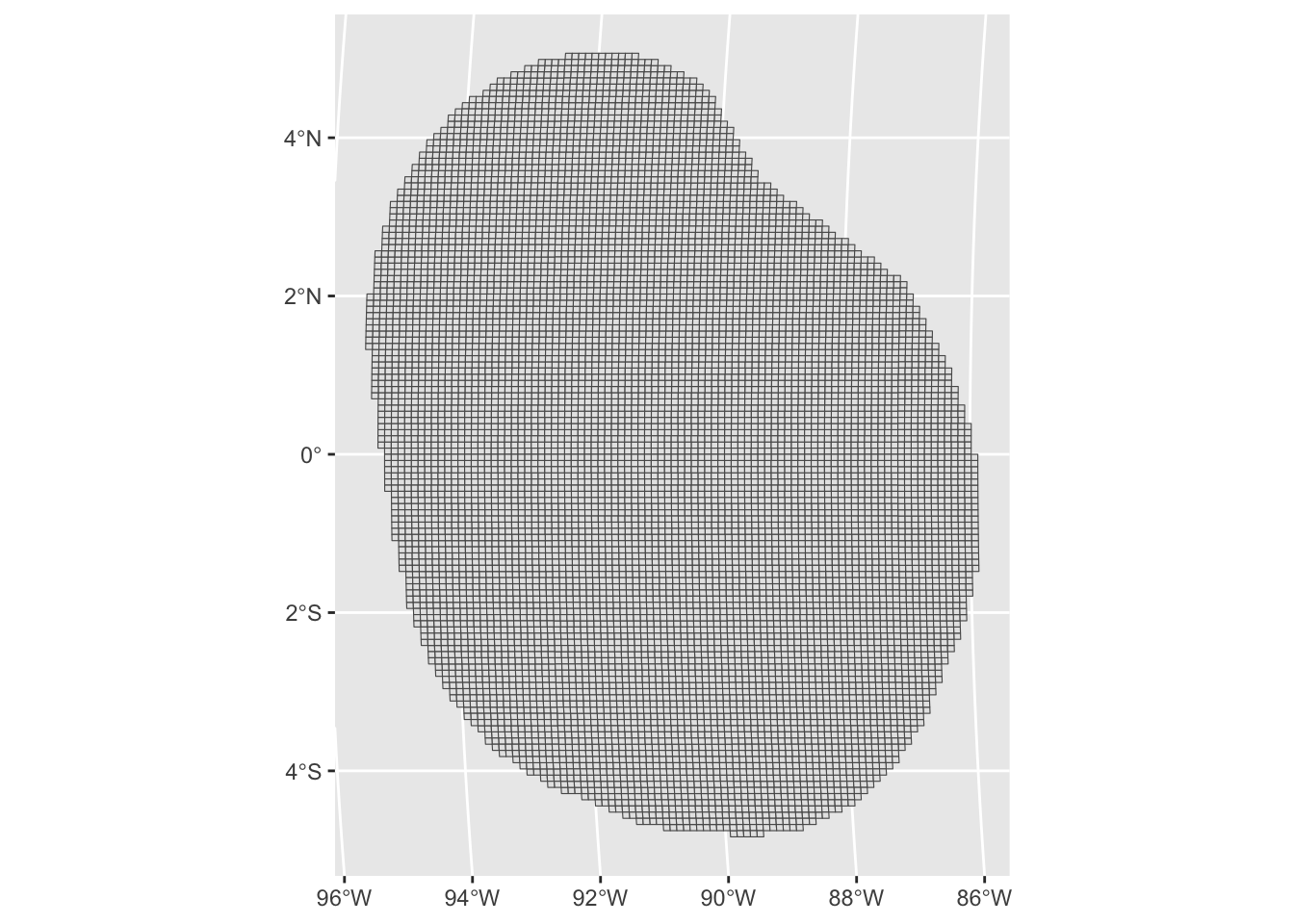

The features object describes the spatial distribution of the features (i.e., the species, habitats or whatever we care about that would have corresponding targets). The feature data are also saved as an sf::st_sf() object. In addition to the cellID and geometry columns, each column corresponds to a feature we are interested in protecting. Values of the features denote the presence (using value of 1) or absence (using value of 0) across the study area.

features <- readRDS(file.path(inputDat, "Features", "Features_Combined.rds"))

Lets have a look at some of the features using ggplot().

ggplot() +
  geom_sf(data = features, aes(fill = tiger_shark))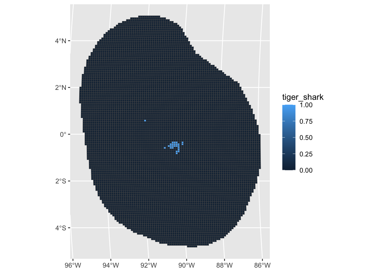

ggplot() +
  geom_sf(data = features, aes(fill = seamount))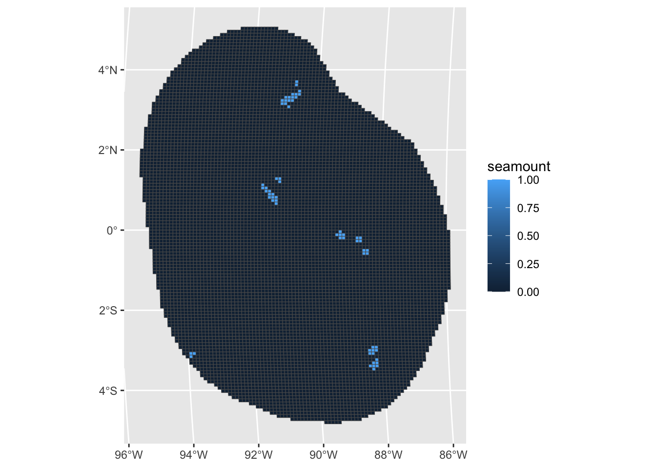

Load Cost

As conservation and management actions are often restricted by costs, we therefore seek to meet targets, while minimizing costs and other impacts on industries, communities or other stakeholders. For this scenario, we will use the cost to the fishing industry. This is a layer that reflects the economic value derived within a given cell for the two primary fishing fleets operating in the Galapagos: the artisanal long-line pelagic fleet, and the industrial tuna purse-seine fleet.

Because there is no fishing allowed in the marine reserve, the cost is negligible and so prioritizr will preference meeting targets in these low-cost areas.

cost <- st_read(file.path(inputDat, "Cost", "cost_surface.shp")) %>%
  st_transform(cCRS) %>%
  rename(cellID = puid)

Reading layer `cost_surface' from data source 
  `/Users/eve067/GitHub/IMCC7_ConsPlanWorkshop/Input/Cost/cost_surface.shp' 
  using driver `ESRI Shapefile'
Simple feature collection with 8749 features and 2 fields
Geometry type: POLYGON
Dimension:     XY
Bounding box:  xmin: -95.42988 ymin: -4.83434 xmax: -85.87651 ymax: 5.068858
Geodetic CRS:  WGS 84

ggplot() +
  geom_sf(data = cost, aes(fill = .data$cost))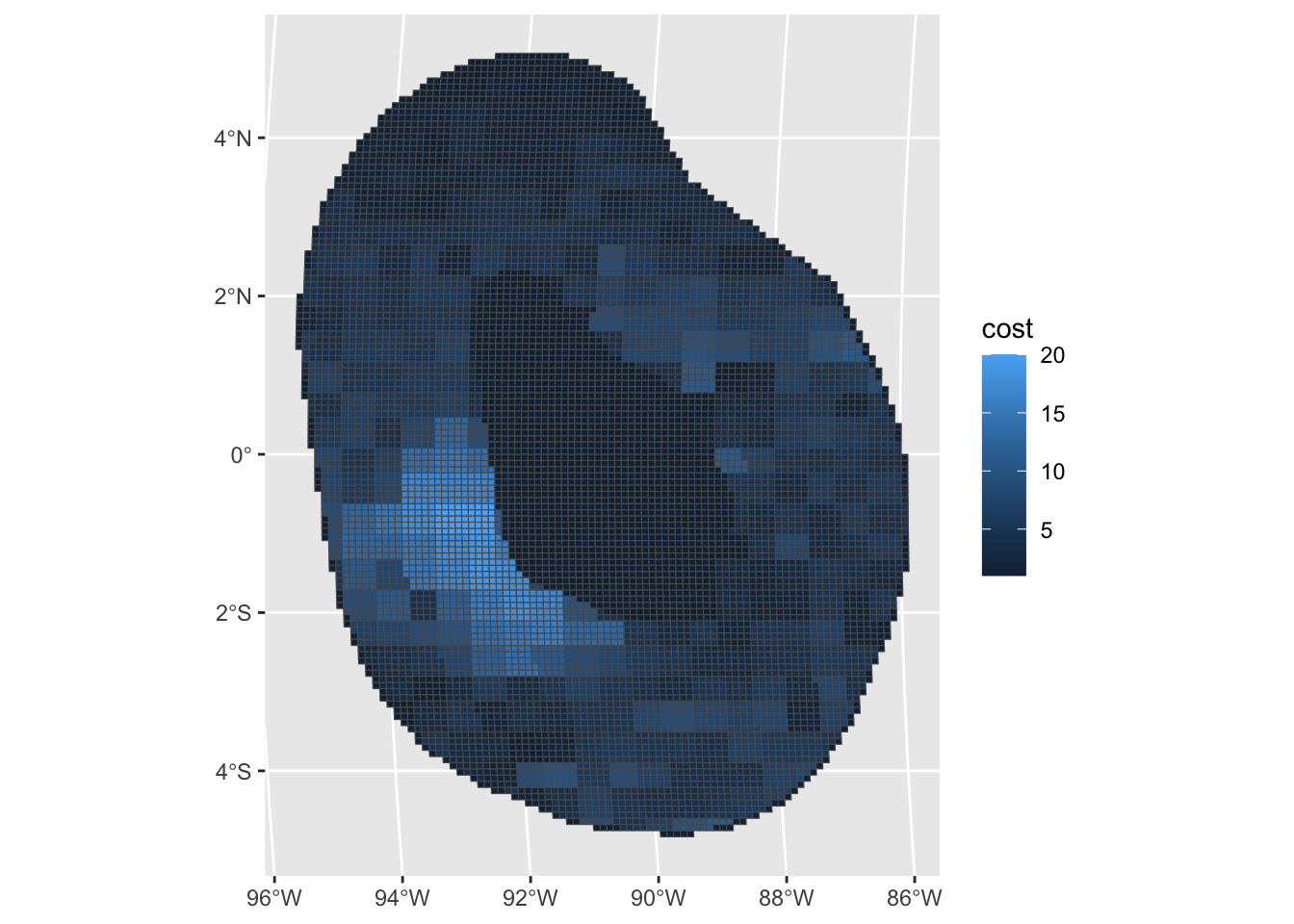

Add cost to combined sf object.

out_sf <- features %>%
  left_join(cost %>% sf::st_drop_geometry(), by = "cellID")

Get the landmass.

landmass <- rnaturalearth::ne_countries(
  scale = "medium",
  returnclass = "sf"
) %>%
  sf::st_transform(cCRS)
landmass <- rnaturalearth::ne_countries(
  scale = "medium",
  returnclass = "sf"
) %>%
  sf::st_transform(cCRS)

Setup prioritization

Now, we do the actual spatial prioritization. We are going to use the R package prioritizr to run the prioritizations. Apart from loading the spatial data, we need to prepare a couple of things for prioritizr. We first need to know the “names” (or their identifiers in the dataset) of the features.

# Extract feature names
col_name <- features %>%
  select(-"cellID") %>%
  st_drop_geometry() %>%
  colnames()

We then need the targets that we are assigning for each feature. Here, we show how we can assign equal targets for all features and how we can also assign different targets for different features. In a practical conservation planning setting, you would set higher targets to features that are more important.

# Same target for all
targets <- rep(0.3, length(col_name))


# Assign higher target for species with tracking data
targets <- data.frame(feature = col_name) %>%
  mutate(Category = c(rep("Geomorphic", 12), rep("Tracking Data", 5))) %>%
  mutate(target = if_else(Category == "Tracking Data", 50 / 100, 5 / 100))

Run prioritsation

We now have all the necessary information needed to run the prioritization. Next, we set up the conservation “problem” using problem() from prioritizr. In this function, we define all the spatial data (i.e., in this example, the object out_sf), what the features are called in out_sf, and the what the cost’s column name is in out_sf. We then use the minimum set objective function to solve this conservation problem (i.e., minimizing the cost while meeting all of the features’ targets) using add_min_set_objective(). We also assign the targets for each of the features using add_relative_targets(). The result of solving this conservation problem would be a binary one (1/0, yes/no, TRUE/FALSE), so the algorithm will assign whether a planning unit has been selected or not selected (using add_binary_decisions()).

dat_problem <- problem(out_sf,
                       features = col_name,
                       cost_column = "cost"
) %>%
  add_min_set_objective() %>%
  add_relative_targets(targets$target) %>%
  add_binary_decisions() %>%
  add_default_solver(verbose = FALSE)

Then, we solve the prioritization using solve.ConservationProblem().

dat_soln <- dat_problem %>%
  solve.ConservationProblem()

And there you have it, you have generated a spatial prioritization! “Solving” the conservation “problem” is a bit anticlimactic, but this shows that most of the work to generate a spatial prioritization is to preprocess and wrangle the spatial data.

If you want to save the output for later use, you can do this in the normal way for R.

saveRDS(dat_soln, file.path("Output", "Solution1.rds"))

Let us plot the solution and see what it looks like.

# Plot solution with a function we have defined (i.e., it is not in prioritizr)
# This makes a prettier plot than using the default plot function in prioritizr
(gg_sol <- splnr_plot_Solution(dat_soln))

Warning: Duplicated `override.aes` is ignored.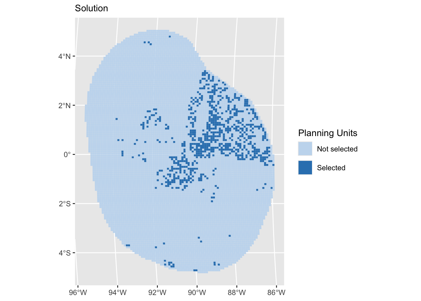

How well were targets met?

targ_coverage <- eval_target_coverage_summary(dat_problem, dat_soln[, "solution_1"])

Irreplaceability

So far, our solution provides information which PUs should be selected to solve the defined conservation problem, so by meeting the targets for the features whilst minimizing the cost. However, some PUs might be more important in contributing to meeting the targets of the features than others. This concept is known as Irreplaceability and essentially measures the value of PUs to achieve the conservation objectives, considering the alternatives.

Prioritizr has three built-in irreplaceability scores that can be applied to the solution to assess the importance of PUs: The Ferrier score, the rarity weighted richness score and the replacement cost score. We have provided code for running all of them, but we will only show the Ferrier score in this workshop, as it is relatively quick to run. Note that this score only works for conservation problems that include targets in their objective and have a single zone.

soln <- dat_soln %>%
  as_tibble()

# Ferrier score
ferrier <- eval_ferrier_importance(dat_problem, soln[, "solution_1"]) %>%
  select("total") %>%
  mutate(geometry = dat_soln$geometry) %>%
  rename(score = "total") %>%
  st_as_sf()

We won’t run these today, but the other two irreplaceability scores are shown here.

# Rarity weighted richness
rwr <- eval_rare_richness_importance(dat_problem, soln[, "solution_1"]) %>%
  mutate(geometry = soln$geometry) %>%
  rename(score = "rwr") %>%
  st_as_sf()

# Replacement cost
replacement <- eval_replacement_importance(dat_problem, soln[, "solution_1"]) %>%
  mutate(geometry = soln$geometry) %>%
  drename(score = "rc") %>%
  st_as_sf()

We can visualise the Ferrier score across the planning domain:

#prep data to allow to see the results better
quant99fs <- round(stats::quantile(ferrier$score, 0.99), 4)
ferrier$score[ferrier$score >= quant99fs] <- quant99fs

# plot results
ggplot() +
  geom_sf(data = ferrier, aes(fill = .data$score), colour = NA)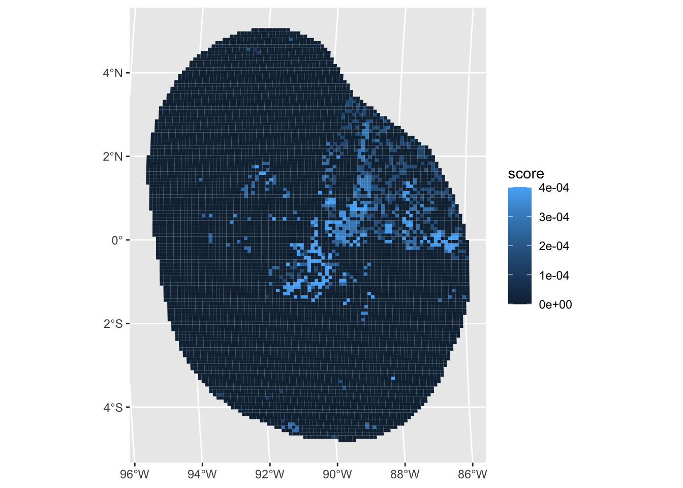

We can see that the majority of PUs has a very low Ferrier score. This means that according to the Ferrier score these PUs are less important than other PUs in terms of meeting all the targets for all features. In contrast, ome PUs in the center of the planning region have a comparably high Ferrier score. This means that not selecting these PUs in the solution would for example require several other PUs for contributing to the targets similarly.

Selection frequency

The algorithm that used to solve conservation problems in prioritizr (integer linear programming), can find optimal solutions to problems. In Marxan, this is not the case, and therefore the term selection frequency is found commonly across literature and practice. The selection frequency represents how many times a PU was selected across a range of solutions, thereby refelecting the importance of PU when meeting targets, but also allowing to explore alternative solutions that might be complementary. In prioritizr, we can also explore the selection frequency by using portfolios.

There are several different portfolio types available in prioritizr. Here, we use add_cuts_portfolio(), which allows to set the number of attempts to generate a different solution. A solution is excluded from the possible solutions to problem after it has previously obtained.

dat_soln_portfolio <- dat_problem %>%
  add_cuts_portfolio(5) %>% # create a portfolio of solutions
  solve.ConservationProblem()

We can now summarize the results to calculate the selection frequency across the 5 attempts and visualize the results.

selFreq <- dat_soln_portfolio %>% # calculate selection frequency
  st_drop_geometry() %>%
  mutate(selFreq = as.factor(rowSums(
   select(., starts_with("solution_"))
  ))) %>%
  st_as_sf(geometry = dat_soln_portfolio$geometry) %>%
  select(selFreq)

ggplot() +
  geom_sf(data = selFreq, aes(fill = .data$selFreq), colour = NA)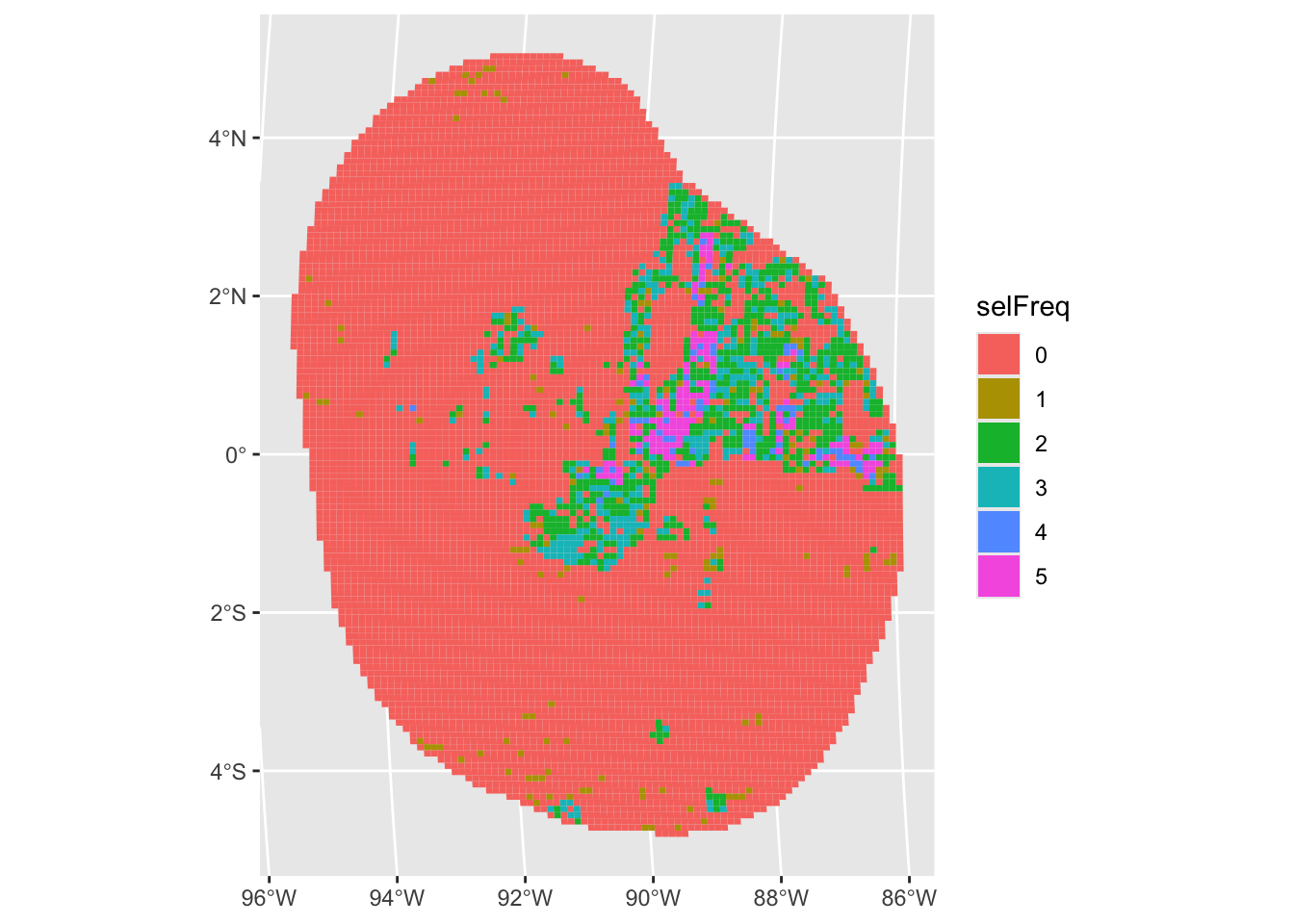

We can see that the majority of PUs have never been selected, some have been selected a few times, and some PUs have even been selected every time. This means these PUs are very important to meet the targets for the features.

Advanced Spatial prioritization

Preliminaries

# Extract feature names

col_name <- features %>%
  select(-"cellID") %>%
  st_drop_geometry() %>%
  colnames()

# Create targets object

# Assign higher target for species with tracking data
targets <- data.frame(feature = col_name) %>%
  mutate(Category = c(rep("Geomorphic", 12), rep("Tracking Data", 5))) %>%
  mutate(target = if_else(Category == "Tracking Data", 50 / 100, 5 / 100))

Create the basic conservation problem

Set up conservation problem.

datEx_problem <- problem(out_sf,
                         features = col_name,
                         cost_column = "cost"
) %>%
  add_min_set_objective() %>% # Add objective function
  add_relative_targets(targets$target) %>% # specify the column with targets
  add_binary_decisions() %>% # Binary answer (Yes/No)
  add_default_solver(verbose = FALSE) # Add solver

# Solve conservation problem
datEx_soln <- datEx_problem %>%
  solve.ConservationProblem() # Solve the problem

Plotting the solution

(gg_soln <- splnr_plot_Solution(datEx_soln) +
   geom_sf(data = landmass, colour = "black", fill = "black", show.legend = FALSE) +
   coord_sf(xlim = st_bbox(PUs)$xlim, ylim = st_bbox(PUs)$ylim))

Coordinate system already present. Adding new coordinate system, which will
replace the existing one.

Warning: Duplicated `override.aes` is ignored.

# How were the targets met?
targetsMet <- eval_feature_representation_summary(
  datEx_problem, 
  datEx_soln[, "solution_1"])

There were a lot of individual PUs selected in the solution. This can be problematic to include in an actual protected area

Adding Penalties

Penalties can be added to the conservation problem as a way to penalize solutions according to a certain metric. Penalizing certain criteria (e.g. certain environmental conditions, activities etc.) leads to a trade-off in the objective function, which aims to minimise the cost. Increasing the “cost” of a planning units through a penalty causes planning units that are not penalized to be selected over those that are.

Penalty 1: Boundary penalty

The boundary penalty helps the user decide how “clumped” the network should be. Often, it is not feasible to enforce a network of fragmented protected areas (as often happens when we optimize with no design constraints). For this reason, we need to adjust the boundary penalty to ensure we can minimize fragmentation and aggregate planning units into patches or clumps. There is no perfect value for the boundary penalty so we encourage users to explore different levels to see the effect.

Set up conservation problem.

datEx_problem_P <- problem(out_sf,
                           features = col_name,
                           cost_column = "cost"
) %>%
  add_min_set_objective() %>%
  add_relative_targets(targets$target) %>%
  add_boundary_penalties(0.5) %>%
  add_binary_decisions() %>%
  add_default_solver(gap = 0.5, verbose = FALSE) # Larger optimality gap to speed up code

Solve conservation problem.

datEx_soln_P <- datEx_problem_P %>%
  solve.ConservationProblem()

(gg_solnP <- splnr_plot_Solution(datEx_soln_P) +
   geom_sf(data = landmass, 
           colour = "black", fill = "black", show.legend = FALSE) +
   coord_sf(xlim = st_bbox(PUs)$xlim, ylim = st_bbox(PUs)$ylim))

Coordinate system already present. Adding new coordinate system, which will
replace the existing one.

Warning: Duplicated `override.aes` is ignored.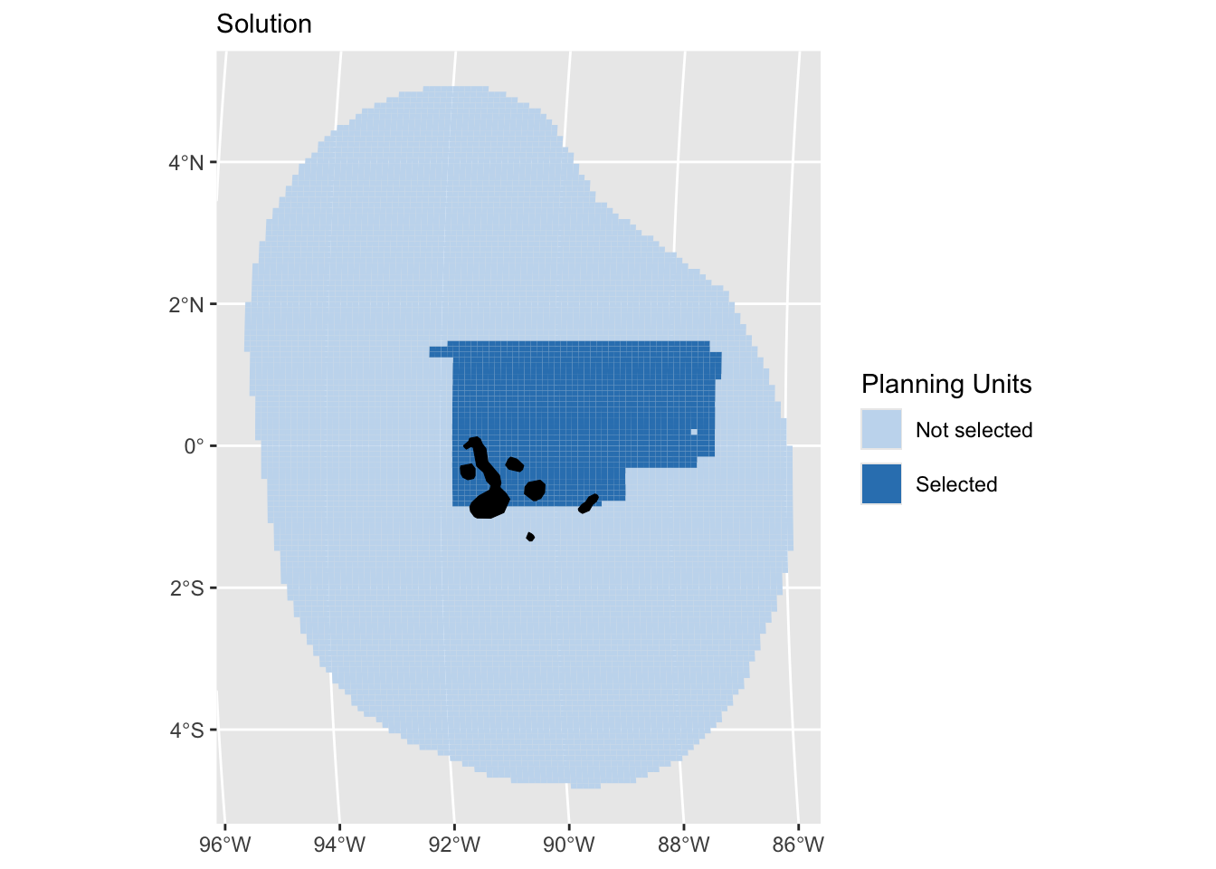

The selected PUs are more aggregated BUT, in an example with varying cost this might also lead to a more expensive solution

Penalty 2: Linear penalty

Another type of penalty is the linear penalty . The linear penalty assumes a linear trade-off between the penalty values and the primary objective of the conservation planning problem (e.g., solution cost for minimum set problems). In our example, we will now set up a conservation problem that uses an area-based primary cost and we will use the fishing information as a penalty, so that selecting values with a high cost are penalized.

# Add another cost for area
out_sf <- out_sf %>%
  mutate(cost_area = rep(1, nrow(.)))

Set up conservation problem.

datEx_problem_linP <- problem(out_sf,
                           features = col_name,
                           cost_column = "cost_area") %>%
  add_linear_penalties(10, data = "cost") %>%
  add_min_set_objective() %>%
  add_relative_targets(targets$target) %>%
  add_binary_decisions() %>%
  add_default_solver(gap = 0.2, verbose = FALSE) # we're adjusting the optimality gap here to speed up the process

Solve conservation problem.

datEx_soln_linP <- datEx_problem_linP %>%
  solve.ConservationProblem()

(gg_solnlinP <- splnr_plot_Solution(datEx_soln_linP) +
    geom_sf(data = landmass, colour = "black", fill = "black", show.legend = FALSE) +
    coord_sf(xlim = st_bbox(PUs)$xlim, ylim = st_bbox(PUs)$ylim))

Coordinate system already present. Adding new coordinate system, which will
replace the existing one.

Warning: Duplicated `override.aes` is ignored.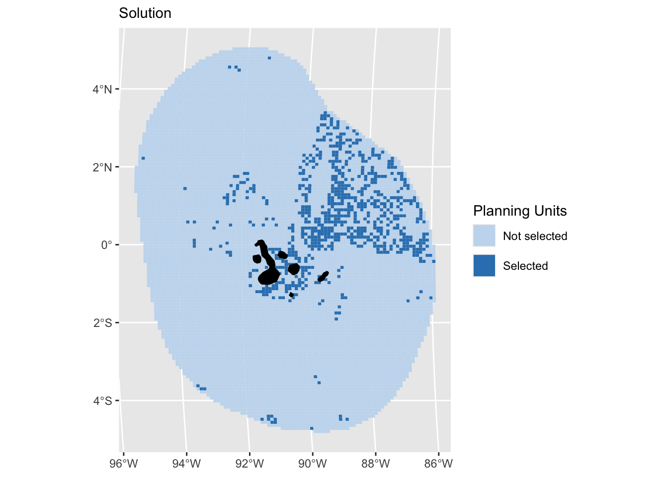

There are several types of penalties, so it is worthwhile browsing through the prioritizr Reference tab for more information.

Adding Constraints

The conservation problems so far were relatively simple. In reality, it is often required to add more complexity. A constraint can be added to a conservation planning problem to ensure that solutions exhibit a specific characteristic.

Constraint 1: Locked-in areas

One example for constraints is locking in specific areas, for example already existing MPAs. These MPA will have to be part of the final solution - after all, they are locked-in.

mpas <- readRDS(file.path(inputDat, "MPAs", "mpas.rds"))

# First look at the data
(gg_mpas <- ggplot() +
    geom_sf(data = mpas, aes(fill = .data$mpas), 
            colour = NA, size = 0.001, show.legend = FALSE))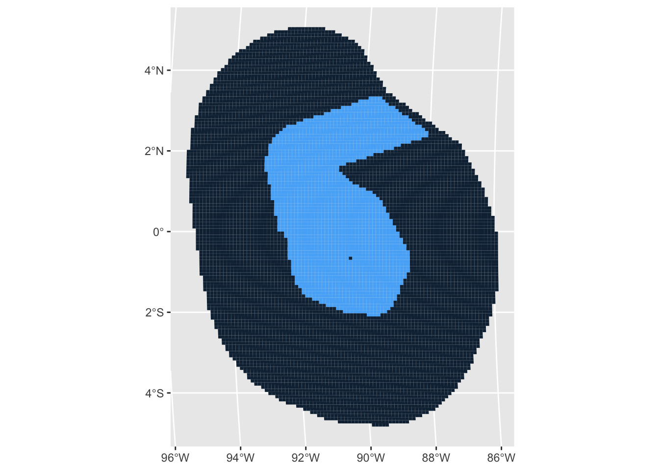

The conservation problem.

datEx_problem_LIC <- problem(out_sf,
                             features = col_name,
                             cost_column = "cost"
) %>%
  add_min_set_objective() %>%
  add_relative_targets(targets$target) %>%
  add_locked_in_constraints(as.logical(mpas$mpas)) %>%
  add_binary_decisions() %>%
  add_default_solver(verbose = FALSE)

# Solve conservation problem
datEx_soln_LIC <- datEx_problem_LIC %>%
  solve.ConservationProblem()

(gg_solnLIC <- splnr_plot_Solution(datEx_soln_LIC) +
    geom_sf(data = landmass, 
            colour = "black", fill = "black", show.legend = FALSE) +
    coord_sf(xlim = st_bbox(PUs)$xlim, ylim = st_bbox(PUs)$ylim))

Coordinate system already present. Adding new coordinate system, which will
replace the existing one.

Warning: Duplicated `override.aes` is ignored.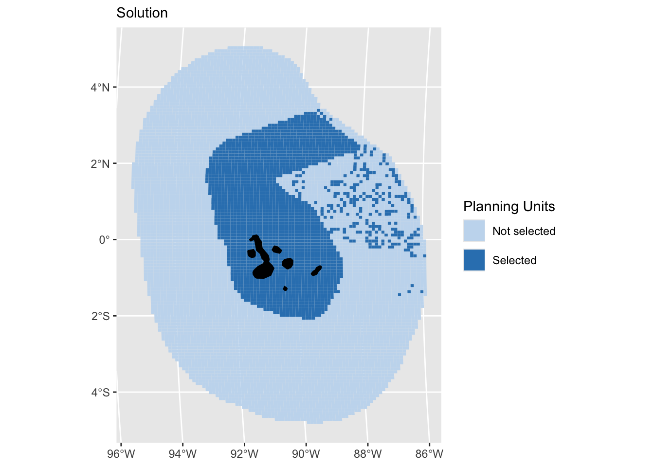

Constraint 2: Linear Constraints

Linear constraints can be used to ensure that solutions meet certain criteria. For example, linear constraints can be used to add multiple budgets or to ensure that the total number of planning units allocated to a certain administrative area (e.g., a bioregion) does not exceed a certain threshold (e.g., 30% of its total area).

# Set up conservation problem
datEx_problem_LC <- problem(out_sf,
                            features = col_name,
                            cost_column = "cost"
) %>%
  add_min_set_objective() %>%
  add_relative_targets(targets$target) %>%
  add_linear_constraints(sum(out_sf$cost_area) * 0.4, 
                         sense = "<=", out_sf$cost_area) %>% # set area-based budget
  add_binary_decisions() %>%
  add_default_solver(verbose = FALSE)

# Solve conservation problem
datEx_soln_LC <- datEx_problem_LC %>%
  solve.ConservationProblem()

(gg_solnLC <- splnr_plot_Solution(datEx_soln_LC) +
    geom_sf(data = landmass, 
            colour = "black", fill = "black", show.legend = FALSE) +
    coord_sf(xlim = st_bbox(PUs)$xlim, ylim = st_bbox(PUs)$ylim))

Coordinate system already present. Adding new coordinate system, which will
replace the existing one.

Warning: Duplicated `override.aes` is ignored.

There are several types of constraints, so it is worthwhile browsing through the prioritizr Reference tab for more information.

Changing Objective Functions

An objective is used to specify the overall goal of a conservation planning problem. All conservation planning problems involve minimizing or maximizing an objective.

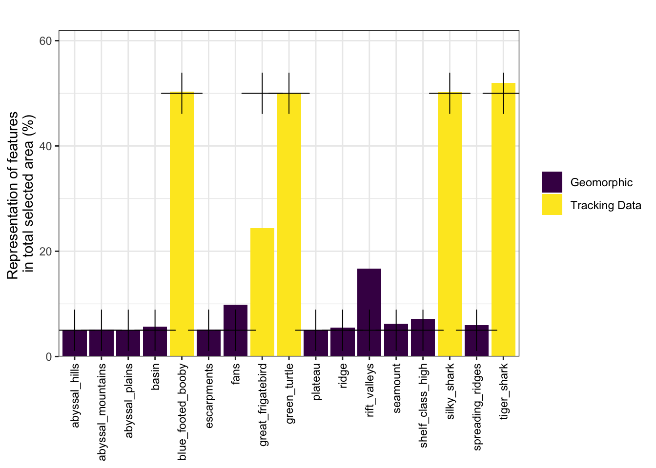
Objective 1: Minimum set

The minimum set objective in a conservation planning problem minimizes the cost of the solution whilst ensuring that all targets are met. This objective is similar to the one used in Marxan.

# Targets
dfTarget <- splnr_get_featureRep(datEx_soln, datEx_problem,
                                 solnCol = "solution_1"
) %>%
  mutate(category = targets$Category)

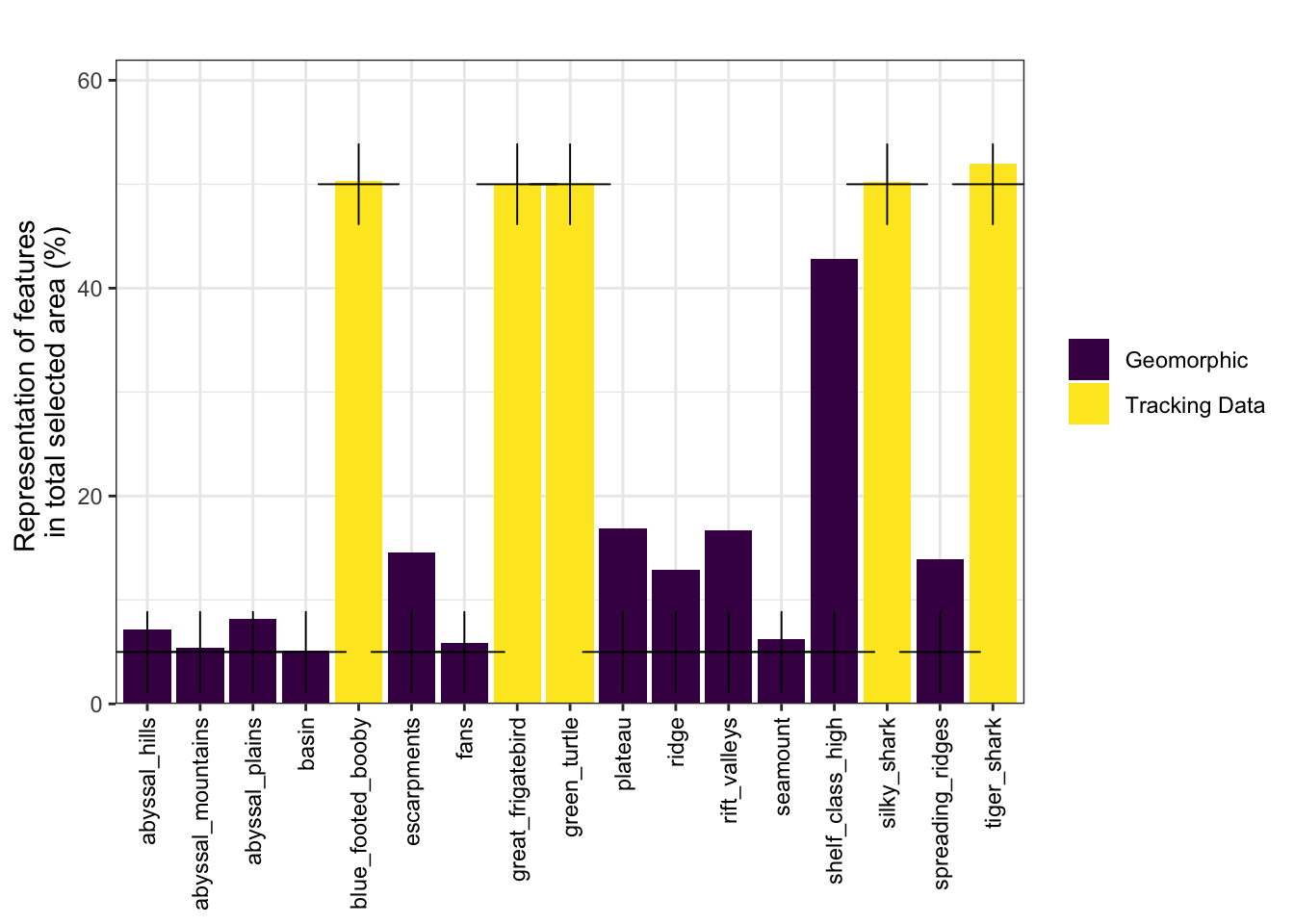
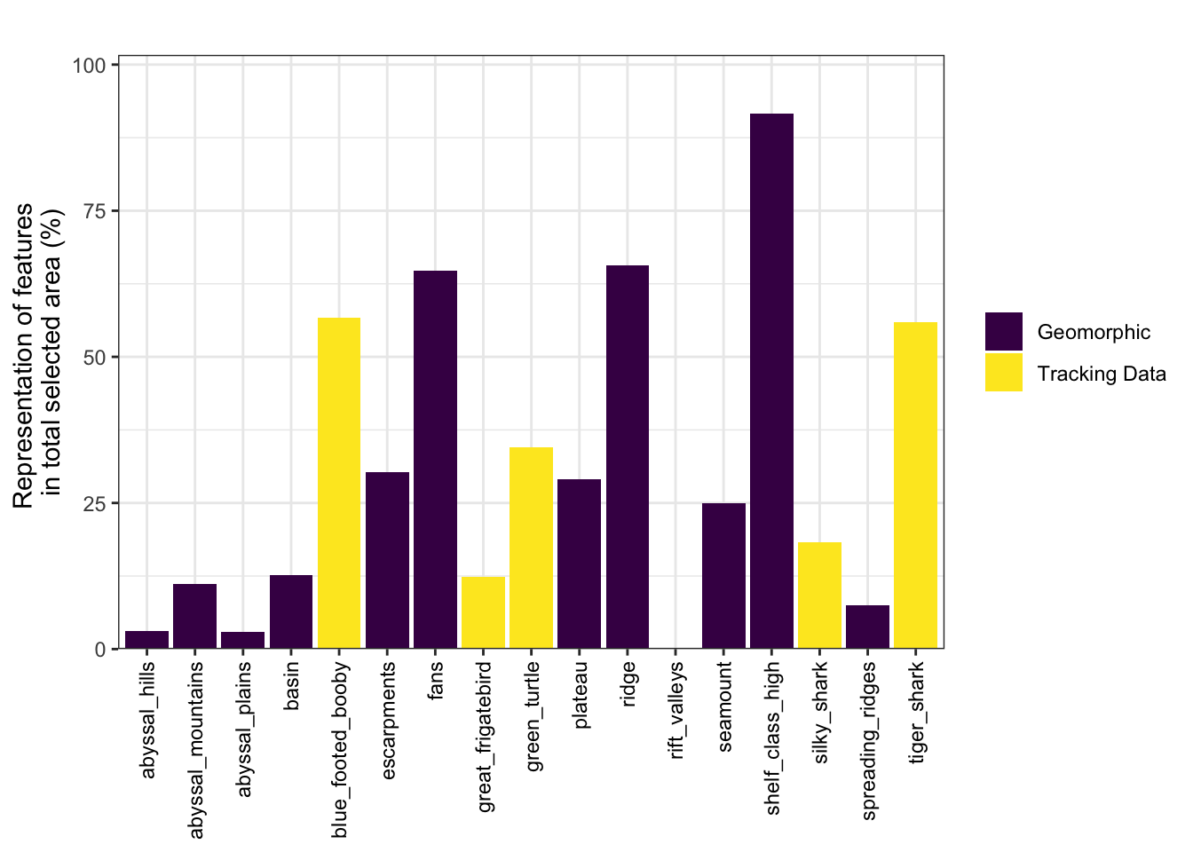
(ggTarget <- splnr_plot_featureRep(
  df = dfTarget,
  nr = 1, showTarget = TRUE
))

Objective 2: Minimum shortfall

The aim of the minimum shortfall objective is to find the set of planning units that minimizes the overall (weighted sum) shortfall for the representation targets. This minimizes the fraction of each target that remains unmet, for as many features as possible while staying within a fixed budget.

# Set up conservation problem
datEx_problem_minS <- problem(out_sf,
                              features = col_name,
                              cost_column = "cost_area"
) %>%
  add_min_shortfall_objective(sum(out_sf$cost_area) * 0.05) %>%
  add_relative_targets(targets$target) %>% # specify column with targets
  add_binary_decisions() %>%
  add_default_solver(verbose = FALSE)

# Solve conservation problem
datEx_soln_minS <- datEx_problem_minS %>%
  solve.ConservationProblem()

(gg_solnminS <- splnr_plot_Solution(datEx_soln_minS) +
    geom_sf(data = landmass, 
            colour = "black", fill = "black", show.legend = FALSE) +
    coord_sf(xlim = st_bbox(PUs)$xlim, ylim = st_bbox(PUs)$ylim))

Coordinate system already present. Adding new coordinate system, which will
replace the existing one.

Warning: Duplicated `override.aes` is ignored.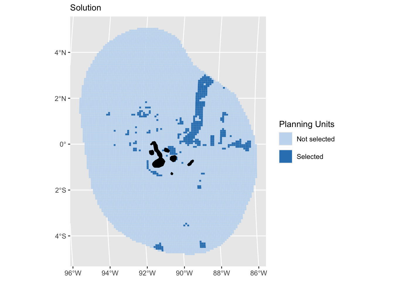

# Feature representation
dfTarget_minS <- splnr_get_featureRep(datEx_soln_minS, datEx_problem_minS,
                                      solnCol = "solution_1"
) %>%
  mutate(category = targets$Category)

(ggTargetminS <- splnr_plot_featureRep(
  df = dfTarget_minS,
  nr = 1, showTarget = TRUE
))

Compare objective functions

(ggTarget_comparison <- ggTarget + ggTargetminS +
   plot_layout(guides = "collect", axes = "collect"))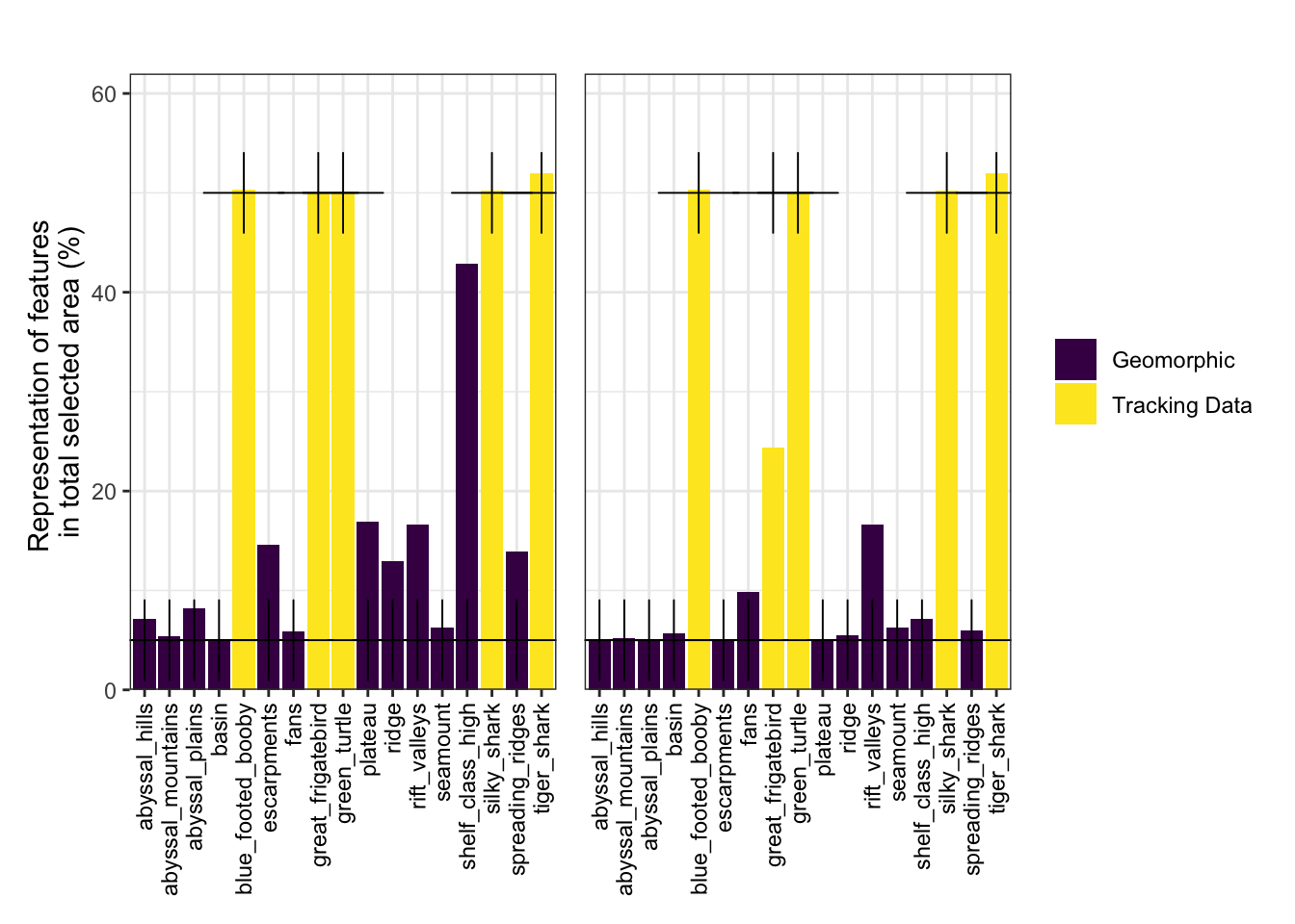

Objective 3: Maximum utility

datEx_problem_maxU <- problem(out_sf,
                              features = col_name,
                              cost_column = "cost_area"
) %>%
  add_max_utility_objective(sum(out_sf$cost_area) * 0.05) %>%
  add_binary_decisions() %>%
  add_default_solver(verbose = FALSE)

# Solve conservation problem
datEx_soln_maxU <- datEx_problem_maxU %>%
  solve.ConservationProblem()

(gg_solnmaxU <- splnr_plot_Solution(datEx_soln_maxU) +
    geom_sf(data = landmass, 
            colour = "black", fill = "black", show.legend = FALSE) +
    coord_sf(xlim = st_bbox(PUs)$xlim, ylim = st_bbox(PUs)$ylim))

Coordinate system already present. Adding new coordinate system, which will
replace the existing one.

Warning: Duplicated `override.aes` is ignored.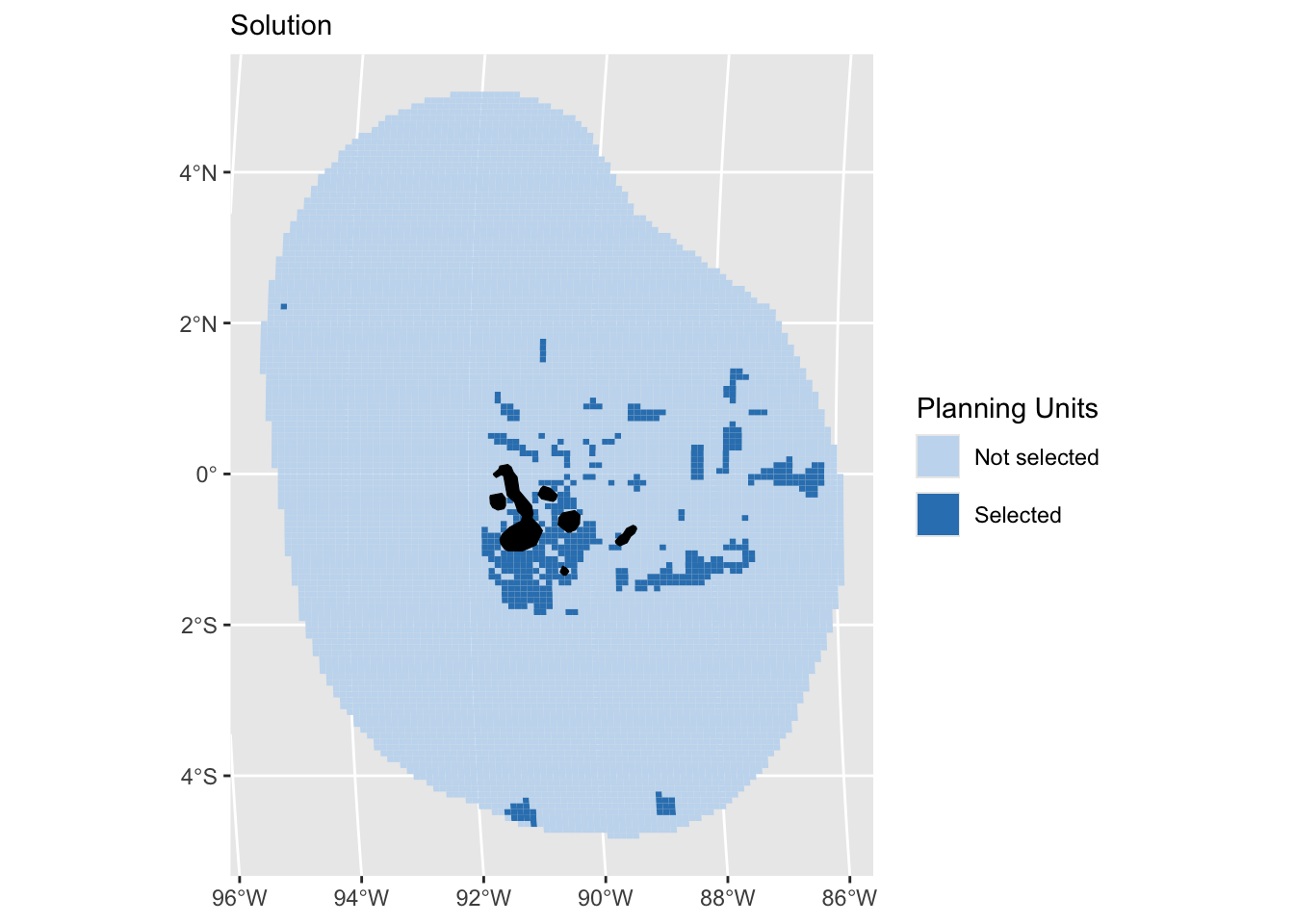

dfTarget_maxU <- splnr_get_featureRep(datEx_soln_maxU, datEx_problem_maxU,
                                      solnCol = "solution_1",
                                      maxUtility = TRUE
) %>%
  mutate(category = targets$Category)

(ggTargetmaxU <- splnr_plot_featureRep(
  df = dfTarget_maxU,
  nr = 1, showTarget = FALSE,
  maxUtility = TRUE
))

We can compare the maximum utility objective function with the minimum set and minimum shortfall objectives.

(ggTarget_comparison2 <- ggTarget + ggTargetminS + ggTargetmaxU +
   plot_layout(guides = "collect", axes = "collect"))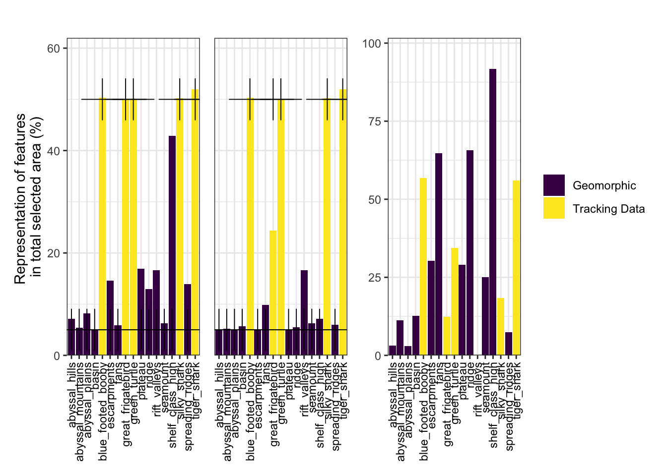

Adding Zones

Many real-world conservation problems do not simply involve deciding if an area should be protected or not. In reality, many problems involve a range of different types of management and the goal is to determine which areas should be allocated to which type of management. We can construct such a conservation problem to have different management zones, using the function zones().

# Create Targets
targetsZones <- data.frame(feature = col_name) %>%
  mutate(Category = c(rep("Geomorphic", 12), rep("Tracking Data", 5))) %>%
  mutate(
    targetZ1 = dplyr::if_else(Category == "Tracking Data", 30 / 100, 0),
    targetZ2 = dplyr::if_else(Category != "Tracking Data", 10 / 100, 0)
  ) %>%
  dplyr::select("targetZ1", "targetZ2") %>%
  as.matrix()

# Create zones object
z1 <- prioritizr::zones("zone 1" = col_name, "zone 2" = col_name)

# Set up conservation problem
# NOTE: when using sf input, we need as many cost columns as we have zones
datEx_problem_zones <- prioritizr::problem(
  out_sf %>%
    mutate(
      Cost1 = rep(1, nrow(.)),
      Cost2 = rep(1, nrow(.))
    ),
  z1,
  cost_column = c("Cost1", "Cost2")
) %>%
  prioritizr::add_min_set_objective() %>%
  prioritizr::add_relative_targets(targetsZones) %>%
  prioritizr::add_binary_decisions() %>%
  prioritizr::add_default_solver(verbose = FALSE)

# Solve conservation problem
datEx_soln_zones <- datEx_problem_zones %>%
  prioritizr::solve.ConservationProblem()

We can examine the solution.

(gg_soln_zones <- splnr_plot_Solution(
  datEx_soln_zones,
  zones = TRUE,
  colorVals = c("#c6dbef", "#3182bd", "#003366"),
  legendLabels = c("Not selected", "Zone 1", "Zone 2")
) +
  geom_sf(data = landmass, 
          colour = "black", fill = "lightgrey", show.legend = FALSE) +
  coord_sf(xlim = st_bbox(PUs)$xlim, ylim = st_bbox(PUs)$ylim))

Coordinate system already present. Adding new coordinate system, which will
replace the existing one.

Warning: Duplicated `override.aes` is ignored.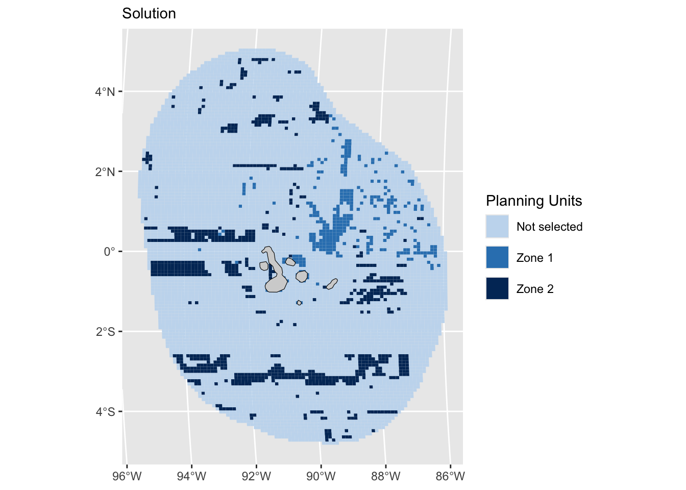

# Feature representation
targetsMet_zones <- datEx_soln_zones %>%
  dplyr::select(tidyselect::starts_with(c("solution"))) %>%
  sf::st_drop_geometry() %>%
  tibble::as_tibble() %>%
  prioritizr::eval_feature_representation_summary(datEx_problem_zones, .)

Beyond code - Apps and communication

Opening up conservation planning to a wider audience: communicating results effectively and transparently to stakeholders and managers using R Shiny Apps and MaPP

Concluding Remarks

References

Acuña-Marrero, D., Smith, A.N.H., Hammerschlag, N., Hearn, A., Anderson, M.J., Calich, H., Pawley, M.D.M., Fischer, C., Salinas-de-León, P., 2017. Residency and movement patterns of an apex predatory shark (Galeocerdo cuvier) at the Galápagos Marine Reserve. PLoS One 12, e0183669.

Galapagos Movement Consortium, Movebank Data Repository https://www.movebank.org/cms/movebank-main

Harris, P.T., Macmillan-Lawler, M., Rupp, J. and Baker, E.K., 2014. Geomorphology of the oceans. Marine Geology, 352, pp.4-24.

Hearn, A.R., Acuña, D., Ketchum, J.T., Peñaherrera, C., Green, J., Marshall, A., Guerrero, M., Shillinger, G., 2014. Elasmobranchs of the Galápagos Marine Reserve, In (J. Denkinger, L. Vinueza, eds.) Galápagos Marine Reserve: a dynamic socio-ecological system., pp. 23-59. Springer.

Hearn, A.R., Green, J., Román, M.H., Acuña-Marrero, D., Espinoza, E., Klimley, A.P., 2016. Adult female whale sharks make long-distance movements past Darwin Island (Galápagos, Ecuador) in the Eastern Tropical Pacific. Marine Biology 163, 214.

Hearn, A.R., Espinoza, E., Ketchum, J., Green, J., Peñaherrera, C., Arauz, R., Fischer, C., Steiner, T., Shillinger, G., Henderson, S., Bessudo, S., Soler, G., Klimley, P., 2017. Una década de seguimiento de los movimientos de tiburones resalta la importancia ecológica de las islas del norte: Darwin y Wolf, In (L. Cayot, D. Cruz, eds.) Informe Galápagos 2015-2016. pp. 132-142. DPNG, CGREG, FCD & GC, Puerto Ayora, Galápagos, Ecuador.

Hearn A, Cárdenas S, Allen H, Zurita L, Gabela-Flores MV, Peñaherrera-Palma CR, Castrejón M, Cruz S, Kelley D, Jeglinski J, Bruno J, Jones J, Naveira-Garabato A, Forryan A, Viteri C, Picho J, Donnelly A, Tudhope A, Wilson M & G Reck G (2022). A Blueprint for Marine Spatial Planning of Ecuador’s Exclusive Economic Zone around the Galápagos Marine Reserve. Universidad San Francisco de Quito / PEW Bertarelli Ocean Legacy, Quito, Ecuador, 361 p.

Parra, D.M., Andrés, M., Jiménez, J., Banks, S., Muñoz, J.P., 2013. Evaluación de la incidencia de impacto de embarcaciones y distribución de la tortuga verde (Chelonia mydas) en Galápagos. Retrieved from Puerto Ayora, Galapagos, Ecuador

Seminoff, J.A., Zárate, P., Coyne, M., Foley, D.G., Parker, D., Lyon, B.N., Dutton, P.H., 2008. Post-nesting migrations of Galápagos green turtles Chelonia mydas in relation to oceanographic conditions: integrating satellite telemetry with remotely sensed ocean data. Endangered Species Research 4, 57-72

Shillinger, G.L., Swithenbank, A.M., Bailey, H., Bograd, S.J., Castelton, M.R., Wallace, B.P., Spotila, J.R., Paladino, F.V., Piedra, R., Block, B.A., 2011. Vertical and horizontal habitat preferences of post-nesting leatherback turtles in the South Pacific Ocean. Marine Ecology Progress Series 422, 275-289.